

Excel makes it easy to crunch numbers. With Excel, you can streamline data entry with AutoFill. Then, get chart recommendations based on your data, and create them with one click. Or easily spot trends and patterns with data bars, colour coding, and icons.
This article is under further development
Learn what Excel is
Excel makes it easy to crunch numbers. With Excel, you can streamline data entry with AutoFill. Then, get chart recommendations based on your data, and create them with one click. Or easily spot trends and patterns with data bars, color coding, and icons.
Click here to watch an introduction video about Excel
-
Open Excel.
-
Go to File. Select Blank workbook.
Or press Ctrl+N.
Enter data
To manually enter data:
-
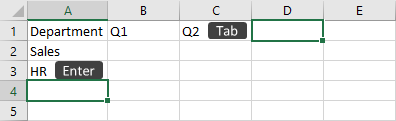
Select an empty cell, such as A1, and then type text or a number.
-
Press Enter or Tab to move to the next cell.
To fill data in a series:
-
Enter the beginning of the series in two cells: such as Jan and Feb; or 2014 and 2015.
-
Select the two cells containing the series, and then drag the fill handle
 across or down the cells.

^ Go to top
Save your workbook to OneDrive in Excel
Save a workbook to OneDrive to access it from different devices and share and collaborate with others.
-
Select File > Save As.
-
For work or school, select
OneDrive - <Company name>. -
For personal files, select
OneDrive - Personal.
-
-
Enter a file name and select Save.
Note:
You may need to sign in to your account.
^ Go to top
Enter and format data
Change the column width
If you find yourself needing to expand or reduce Excel's column widths, there are several ways to adjust them.
Set a column to a specific width
-
Select the column or columns that you want to change.
-
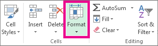
On the Home tab, in the Cells group, click Format.
-
Under Cell Size, click Column Width.
-
In the Column width box, type the value that you want.
-
Click OK.
Tip: To quickly set the width of a single column, right-click the selected column, click Column Width, type the value that you want, and then click OK.
Change the column width to automatically fit the contents using Autofit
-
Select the column or columns that you want to change.
-
On the Home tab, in the Cells group, click Format.
-
Under Cell Size, click AutoFit Column Width.
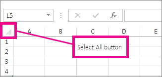
Note: To quickly autofit all columns on the worksheet, click the Select All button, and then double-click any boundary between two column headings.
Match the column width to another column
-
Select a cell in the column that has the width that you want to use.
-
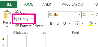
Press Ctrl+C, or on the Home tab, in the Clipboard group, click Copy.
-
Right-click a cell in the target column, point to Paste Special, and then click the Keep Source Columns Widths
 button.
Change the default width for all columns on a worksheet or workbook
The value for the default column width indicates the average number of characters of the standard font that fit in a cell. You can specify a different number for the default column width for a worksheet or workbook.
-
Do one of the following:
-
To change the default column width for a worksheet, click its sheet tab.
-
To change the default column width for the entire workbook, right-click a sheet tab, and then click Select All Sheets on the shortcut menu.
-
-
On the Home tab, in the Cells group, click Format.
-
Under Cell Size, click Default Width.
-
In the Standard column width box, type a new measurement, and then click OK.
Change the width of columns by using the mouse
Do one of the following:
-
To change the width of one column, drag the boundary on the right side of the column heading until the column is the width that you want.
-
To change the width of multiple columns, select the columns that you want to change, and then drag a boundary to the right of a selected column heading.
-
To change the width of columns to fit the contents, select the column or columns that you want to change, and then double-click the boundary to the right of a selected column heading.
To change the width of all columns on the worksheet, click the Select All button, and then drag the boundary of any column heading.
If you find yourself needing to expand or reduce Excel's row widths and column heights, there are several ways to adjust them.
Set row to a specific height
-
Select the row or rows that you want to change.
-
On the Home tab, in the Cells group, click Format.
-
Under Cell Size, click Row Height.
In the Row height box, type the value that you want, and then click OK.
Change the row height to fit the contents
-
Select the row or rows that you want to change.
-
On the Home tab, in the Cells group, click Format.
-
Under Cell Size, click AutoFit Row Height.
Tip: To quickly autofit all rows on the worksheet, click the Select All button, and then double-click the boundary below one of the row headings.
Change the height of rows by using the mouse
Do one of the following:
-
To change the row height of one row, drag the boundary below the row heading until the row is the height that you want.
-
To change the row height of multiple rows, select the rows that you want to change, and then drag the boundary below one of the selected row headings.
-
To change the row height for all rows on the worksheet, click the Select All button, and then drag the boundary below any row heading.
-
To change the row height to fit the contents, double-click the boundary below the row heading.
Move or copy cells, rows, and columns
In the Windows version of Excel: you can use the Cut command or Copy command to move or copy selected cells, rows, and columns, but you can also move or copy them by using the mouse.
Move or copy rows and columns by using commands
-
Select the cell, row, or column that you want to move or copy.
-
Do one of the following:
-
To move rows or columns, on the Home tab, in the Clipboard group, click Cut
 or press CTRL+X.
 -
To copy rows or columns, on the Home tab, in the Clipboard group, click Copy
 or press CTRL+C.
-
-
Right-click a row or column below or to the right of where you want to move or copy your selection, and then do one of the following:
Tip:
To move or copy a selection to a different worksheet or workbook, click another worksheet tab or switch to another workbook, and then select the upper-left cell of the paste area.-
When you are moving rows or columns, click Insert Cut Cells.
-
When you are copying rows or columns, click Insert Copied Cells.
-
Note:
Excel displays an animated moving border around cells that were cut or copied. To cancel a moving border, press Esc.
Move or copy rows and columns by using the mouse
-
Select the row or column that you want to move or copy.
- Do one of the following:
Note:
Make sure that you hold down CTRL or SHIFT during the drag-and-drop operation. If you release CTRL or SHIFT before you release the mouse button, you will move the rows or columns instead of copying them.
-
Cut and replace Point to the border of the selection. When the pointer becomes a move pointer
 , drag the rows or columns to another location. Excel warns you if you are going to replace a column. Press Cancel to avoid replacing.
-
Copy and replace Hold down CTRL while you point to the border of the selection. When the pointer becomes a copy pointer
 , drag the rows or columns to another location. Excel doesn't warn you if you are going to replace a column. Press CTRL+Z if you don't want to replace a row or column.
-
Cut and insert Hold down SHIFT while you point to the border of the selection. When the pointer becomes a move pointer
, drag the rows or columns to another location.
-
Copy and insert Hold down SHIFT and CTRL while you point to the border of the selection. When the pointer becomes a move pointer
, drag the rows or columns to another location.
Note:
You cannot move or copy nonadjacent rows and columns by using the mouse.
Move or copy just the contents of a cell
-
Double-click the cell that contains the data that you want to move or copy. You can also edit and select cell data in the formula bar.
-
Select the row or column that you want to move or copy.
-
On the Home tab, in the Clipboard group, do one of the following:
-
To move the selection, click Cut
or press Ctrl+X.
-
To copy the selection, click Copy
or press Ctrl+C.
-
-
In the cell, click where you want to paste the characters, or double-click another cell to move or copy the data.
-
On the Home tab, in the Clipboard group, click Paste
 or press Ctrl+V.
Press ENTER.
Note:
When you double-click a cell or press F2 to edit the active cell, the arrow keys work only within that cell. To use the arrow keys to move to another cell, first press Enter to complete your editing changes to the active cell.
Copy cell values, cell formats or formulas only
When you paste copied data, you can do any of the following:
-
Paste only the cell formatting, such as font color or fill color (and not the contents of the cells).
-
Convert any formulas in the cell to the calculated values without overwriting the existing formatting.
-
Paste only the formulas (and not the calculated values).
Procedure
-
Select the row or column that you want to move or copy.
-
On the Home tab, in the Clipboard group, click Copy
or press Ctrl+C.
-
Select the upper-left cell of the paste area or the cell where you want to paste the value, cell format, or formula.
-
On the Home tab, in the Clipboard group, click the arrow below Paste
, and then do one of the following:
-
To paste values only, click Values.
-
To paste cell formats only, click Formatting.
-
To paste formulas only, click Formulas.
-
Copy cell width settings
When you paste copied data, the pasted data uses the column width settings of the target cells. To correct the column widths so that they match the source cells, follow these steps.
-
Select the row or column that you want to move or copy.
-
On the Home tab, in the Clipboard group, do one of the following:
-
To move cells, click Cut
or press Ctrl+X.
-
To copy cells, click Copy
or press Ctrl+C.
-
-
Select the upper-left cell of the paste area.
Tip:
To move or copy a selection to a different worksheet or workbook, click another worksheet tab or switch to another workbook, and then select the upper-left cell of the paste area.
On the Home tab, in the Clipboard group, click the arrow under Paste , and then click Keep Source Column Widths.
Note:
When you move or copy rows and columns, by default Excel moves or copies all data that they contain, including formulas and their resulting values, comments, cell formats, and hidden cells.
When you copy cells that contain a formula, the relative cell references are not adjusted. Therefore, the contents of cells and of any cells that point to them might display the #REF! error value. If that happens, you can adjust the references manually. For more information, see Detect errors in formulas.
Contact: Information Systems and Support through case creation.